Introduction to Amazon Bedrock

 

Build Generative AI Applications with Foundation Models - Amazon Bedrock - AWS

Amazon Bedrock is a fully managed service that simplifies the development of generative AI applications using foundation models (FMs) from providers like Anthropic, AI21 Labs, Stability AI, and Amazon itself. 

Key features include:

• Foundation Models: Pre-trained models that can be lightly customized using techniques like fine-tuning or Retrieval Augmented Generation (RAG) without requiring extensive ML expertise.
• Serverless Infrastructure: No need to manage infrastructure; it provides a streamlined, API-based experience for quick deployments
• Security and Privacy: Data is encrypted, region-specific, and not shared with model providers.

Use Cases

Ideal for developers looking to rapidly integrate generative AI into applications such as:

• chatbots
• text generation
• image creation

Cost Model

Pay-as-you-go pricing based on API usage, making it cost-effective for intermittent workloads.

Best for developers or businesses without deep ML expertise who need a fast and easy way to deploy generative AI applications.

Introduction to Large Language Models (LLMs)

Single-turn vs Multi-turn conversation

...

Token

• the smallest unit of text that the model recognizes
• can be a word, a number, or even a punctuation mark
• 1  (English) word has approximately 1.3 tokens

Context Caching

In large language model API usage, a significant portion of user inputs tends to be repetitive. For instance, user prompts often include repeated references, and in multi-turn conversations, previous content is frequently re-entered.

To address this, Context Caching technology caches content that is expected to be reused on a distributed disk array. When duplicate inputs are detected, the repeated parts are retrieved from the cache, bypassing the need for recomputation. This not only reduces service latency but also significantly cuts down on overall usage costs.

Billing

The price of using some LLM is usually in units of per 1M tokens. 

If 1 word has 1.3 tokens, let's see how many words is this: 1w : 1.3t = x : 10^6 => x = 10^6 / 1.3 = 769'230 words ~ 770k words. 

Billing is usually based on the total number of input and output tokens by the model.

If Context Caching is implemented, input billing per 1M tokens can further be split into two categories:

• 1M tokens - Cache Hit (1M tokens that were found in cache)
• 1M tokens - Cache Miss (1M tokens that were not found in cache

Use Case: Chatbots

Chat History

LLMs don't have any concept of state or memory. Any chat history has to be tracked externally and then passed into the model with each new message. We can use a list of custom objects to track chat history. Since there is a limit on the amount of content that can be processed by the model, we need to prune the chat history so there is enough space left to handle the user's message and the model's responses. Our code needs to delete older messages.

Retrieval-Augmented Generation (RAG)

If the responses from the chatbot are based purely on the underlying foundation model (FM), without any supporting data source, they can potentially include made-up responses (hallucination). 

Retrieval-augmented generation LLMs create a more powerful chatbots that incorporates the retrieval-augmented generation pattern to return more accurate responses.

...

Resources:

Building with Amazon Bedrock

Introduction to VertexAI

Vertex AI

• Google's managed machine learning platform
• Designed to help developers, data scientists, and businesses:
• build
• deploy
• scale machine learning models
• Provides a comprehensive suite of tools for every stage of the machine learning lifecycle, including:
• data preparation
• model training
• evaluation
• deployment
• monitoring

Here’s an overview of what Vertex AI offers:

Key Features of Vertex AI:

1. Unified ML Platform: It consolidates various Google AI services into one integrated platform, making it easier to manage end-to-end workflows.

2. Custom and Pre-trained Models:

   • You can train your custom machine learning models using your own data.
   • Alternatively, use Google’s pre-trained models or APIs for common AI tasks (e.g., Vision AI, Translation AI, and Natural Language AI).

3. AutoML:

   • Offers an automated way to train machine learning models, making it accessible even to those without deep expertise in ML.

4. Notebooks:

   • Managed Jupyter Notebooks are available for building and experimenting with ML models.

5. Data Preparation and Labeling:

   • Tools for managing datasets, preparing data, and labeling it for supervised learning tasks.

6. Training and Tuning:

   • Supports large-scale training with powerful infrastructure and features like hyperparameter tuning for optimizing models.

7. Model Deployment:

   • Seamlessly deploy models to an endpoint for real-time predictions or batch processing.

8. Model Monitoring:

   • Tracks the performance of deployed models, monitoring metrics such as prediction drift or latency.

9. Integration with BigQuery and Google Cloud Services:

   • Easily access and analyze data stored in BigQuery and integrate it with other Google Cloud services.

10. ML Ops Features:

    • Tools for managing and automating ML workflows, like pipelines and version control for reproducibility.

Why Use Vertex AI?

• Scalability: It handles infrastructure concerns so you can focus on model development.
• Ease of Use: Tools like AutoML simplify machine learning for those with less technical expertise.
• Cost-Effectiveness: Pay-as-you-go pricing lets you control costs.
• Integration: Works seamlessly with Google Cloud services, making it a powerful choice for businesses already in the Google ecosystem.

It’s ideal for both beginners looking for simplicity and experts needing advanced tools and customizability.

Unsupervised Machine Learning

Data is, by default, unlabeled. Labeling data is manual (or somewhat automated) process, thus timely and expensive. Unsupervised machine learning uses unlabeled data (raw, cheap, widely available) for model training. Nevertheless, this comes with the cost of unsupervised learning requiring higher volumes of data for the training if comparing to supervised learning.

Typical use cases for unsupervised ML:

• Clustering
• Anomaly Detection
• Dimensionality Reduction

Clustering

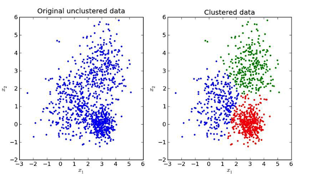
Unsupervised learning algorithms extract features and patterns from unlabeled data which can then be used to label and group together data points that share same or similar features. This is known as clustering and is one of typical problems solved by unsupervised learning.

image source: KDNuggets

Clustering algorithms:

• k-means clustering
• neural networks
• hypothesis function is a mapping from input space back into this input space
• the goal of an unsupervised learning loss function is to measure the difference between the hypothesis function and the input itself

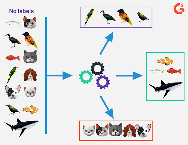
Example: Image set clustering

Each cluster contains images which have the same object in them. Model does not know the name of that object, that it is e.g. bird. It only knows (learns) that objects in each cluster share the same/similar features. We might only need to set in advance the number of clusters we want to get.

In supervised learning, if we have a labeled dataset which contains images of birds, fish and mammals, our model will learn to identify if the image contains a bird, a fish or a mammal. In unsupervised learning, model will learn to distinguish and separate images that share same/similar features and it would group them in three clusters but it would not know that in one cluster are birds and in another fish for example, it would just know that there are three (or maybe even more) types of objects. 

image credits: Devin Pickell, g2.com

Example: Customer segmentation

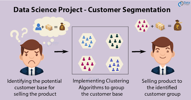
Each cluster contains customers of some differentiable profile. This helps in e.g. targeted marketing.

image source: data-flair.training

Example: Spam detection

Unsupervised learning algorithm can analyze huge volumes of emails and uncover the features and patterns that indicate spam (and keep getting better at flagging spam over time).

Anomaly Detection

Another type of problems solved by unsupervised learning is anomaly detection. The goal here is to find abnormal data points. Model is trained to detect if data point has some unusual features.

Example: Fraud detection (Anomaly Detection)

Fraudulent transactions tend to involve larger sums of money. Fraud only occurs with transfers and cash-out transactions.

image credit: Shirin Elsinghorst, codecentric.de

Class 0 is normal transaction. Class 1 is fraudulent transaction.

Dimensionality Reduction

Data dimensionality refers to feature space. Each data point can be defined as a vector in N-dimensional space where N is number of features. Some features are more and some less important, in a way how much do they contribute in differentiating data points. The more features, the more complex model is, the more time and storage is required for its training and inference. The idea here is to reduce number of features without losing the semantic meaning of the data. E.g. bird can still be distinguished from other animals by recognising that it has features like beak, wings and a tail but eye color or feather color pattern is not important.

Some dimensionality reduction techniques:

• Independent Components Analysis (ICA)
• Principal Components Analysis (PCA)

Sometimes, before applying k-means clustering, a dimensionality reduction is applied on data.

Principal Component Analysis (PCA)

Transforms data from d-dimensional to p-dimensional feature space where p < d. It first finds the dimension of the highest variance (e.g. direction where the data is most spread out) - principal component. Data points are then projected onto this dimension. Small amount of information gets lost but overall data integrity is not changed.

PCA is based on reducing correlation (linear dependence) between features. If two features are linearly dependent, we can derive value of one feature if value of the another one is known. PCA removes this redundancy by projecting a set of linearly dependent features into a smaller set of new, uncorrelated features. 

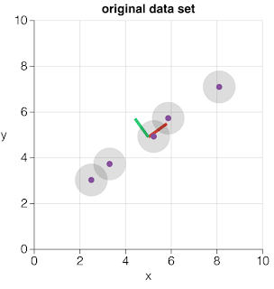
Original data points are in 2-dimensional feature space. Features are denoted as x and y.
 

PCA finds the direction along which values have the highest variance. It is a red diagonal in our case.

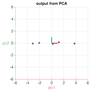
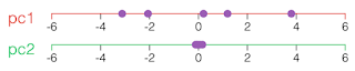
Data points are projected onto component which carries the highest variance. That principal component becomes a newly derived feature. The next principal component (pc2) which carries the most variance is the one defined by the line perpendicular to the direction of pc1.

As pc2 exhibits low variance, this component does not carry much information (that helps differentiating data points). It can be ignored (small amount of information is lost) thus reducing the feature space to a single dimension.

image credits: V. Powell, setosa.io

Example: Solution to “Cocktail Party” problem

Dimension Reduction via Independent Components Analysis (ICA) is used to extract independent sources of audio signal from a recording which contains mixed signals.

image source: 2014, J. Shlens: "A Tutorial on Independent Component Analysis"

References

Unsupervised learning - Wikipedia

Supervised vs Unsupervised Learning – What's the Difference?

Data Science Project - Customer Segmentation using Machine Learning in R - DataFlair

Data Science for Fraud Detection - codecentric AG Blog

[PDF] A Tutorial on Independent Component Analysis | Semantic Scholar

Unsupervised learning

Commonly Used Machine Learning Algorithms | Data Science

Unsupervised Learning Definition | DeepAI

(203) Can deep convolutional neural network be trained via unsupervised learning? - Quora

Principal Component Analysis (PCA)— Part 1 — Fundamentals and Applications | by Nitish Kumar Thakur | Analytics Vidhya | Medium

Principal Component Analysis explained visually

(206) What is principal component analysis and how many variables can be used for PCA? - Quora

Introduction to Principal Component Analysis(PCA) - AI ASPIRANT

Running NVIDIA DIGITS Docker container on Ubuntu

Installing NVIDIA DIGITS directly on your computer means that you'll:

• spend a considerable amount of time in installing all dependencies and building DIGITS itself
• pollute your machine with another application and its dependencies

To prevent this, we can run NVIDIA DIGITS Docker container. Let's check first whether docker is installed and its version :

$ docker --version

Docker version 20.10.3, build 48d30b5

For the reference, I was running the commands I listed below in this article on my Ubuntu 20.04:

$ lsb_release -a

No LSB modules are available.

Distributor ID: Ubuntu

Description: Ubuntu 20.04.2 LTS

Release: 20.04

Codename: focal

Ideally, we'd be running NVIDIA Digits on a machine with GPU(s). This would speed up training and inference but Digits can also work on a machine which has a CPU only. 

I have GeForce GT 640 graphics card:

$ nvidia-smi -L

GPU 0: GeForce GT 640 (UUID: GPU-f2583df9-404d-2564-d332-e7878a94d087)

$ lspci

...

VGA compatible controller: NVIDIA Corporation GK107 [GeForce GT 640 OEM] (rev a1)

...

GK107 is a code name for GeForce GT 640 (GDDR5) (source: GeForce 600 series - Wikipedia) which, according to CUDA GPUs | NVIDIA Developer, has computing capability 3.5 (which is supported as it has to be >2.1 according to Installation Guide — NVIDIA Cloud Native Technologies documentation).

To test the local GPU we can run nvidia-smi application on the local host or in Docker image.

If we haven't installed CUDA or nvidia-smi locally, we can run nvidia-smi from NVIDIA CUDA Docker image:

$ sudo docker run --rm --gpus all nvidia/cuda:11.0-base nvidia-smi

Thu Feb 11 01:02:09 2021       

+-----------------------------------------------------------------------------+

| NVIDIA-SMI 460.32.03    Driver Version: 460.32.03    CUDA Version: 11.2     |

|-------------------------------+----------------------+----------------------+

| GPU  Name        Persistence-M| Bus-Id        Disp.A | Volatile Uncorr. ECC |

| Fan  Temp  Perf  Pwr:Usage/Cap|         Memory-Usage | GPU-Util  Compute M. |

|                               |                      |               MIG M. |

|===============================+======================+======================|

|   0  GeForce GT 640      Off  | 00000000:01:00.0 N/A |                  N/A |

| 40%   31C    P8    N/A /  N/A |    286MiB /  1992MiB |     N/A      Default |

|                               |                      |                  N/A |

+-------------------------------+----------------------+----------------------+

                                                                               

+-----------------------------------------------------------------------------+

| Processes:                                                                  |

|  GPU   GI   CI        PID   Type   Process name                  GPU Memory |

|        ID   ID                                                   Usage      |

|=============================================================================|

|  No running processes found                                                 |

+-----------------------------------------------------------------------------+

Let's now follow the instructions from DIGITS | NVIDIA NGC. We first need to download the image to our local host:

$ docker pull nvcr.io/nvidia/digits:20.12-tensorflow-py3

20.12-tensorflow-py3: Pulling from nvidia/digits

6a5697faee43: Pulling fs layer 

ba13d3bc422b: Pulling fs layer 

...

cec6045b0d0e: Pulling fs layer 

cb4aa708e833: Waiting 

235cfa23a5f4: Waiting 

24781a3c82ea: Waiting 

f7c7d47c1a97: Pull complete 

...

b57dde2f2923: Pull complete 

Digest: sha256:7542143bc2292fc48a3874786877815a5ca6a74a69366324aaf66914155cb5a7

Status: Downloaded newer image for nvcr.io/nvidia/digits:20.12-tensorflow-py3

nvcr.io/nvidia/digits:20.12-tensorflow-py3

Let's now run the container. docker run has --gpus option which instructs Docker to add GPU devices to container ('all' to pass all GPUs).

$ docker run --gpus all -it --rm nvcr.io/nvidia/digits:20.12-tensorflow-py3

docker: Error response from daemon: could not select device driver "" with capabilities: [[gpu]].

I haven't installed NVIDIA Container Toolkit (nvidia-docker) which enable Docker containers accessing host's GPU. Installation Guide — NVIDIA Cloud Native Technologies documentation describes how to install it:

$ distribution=$(. /etc/os-release;echo $ID$VERSION_ID) \

   && curl -s -L https://nvidia.github.io/nvidia-docker/gpgkey | sudo apt-key add - \

   && curl -s -L https://nvidia.github.io/nvidia-docker/$distribution/nvidia-docker.list | sudo tee /etc/apt/sources.list.d/nvidia-docker.list

$ sudo apt-get update

$ sudo apt-get install -y nvidia-docker2

$ sudo systemctl restart docker

$ nvidia-docker version 

NVIDIA Docker: 2.5.0

Client: Docker Engine - Community

 Version:           20.10.3

 API version:       1.41

 Go version:        go1.13.15

 Git commit:        48d30b5

 Built:             Fri Jan 29 14:33:21 2021

 OS/Arch:           linux/amd64

 Context:           default

 Experimental:      true

Server: Docker Engine - Community

 Engine:

  Version:          20.10.3

  API version:      1.41 (minimum version 1.12)

  Go version:       go1.13.15

  Git commit:       46229ca

  Built:            Fri Jan 29 14:31:32 2021

  OS/Arch:          linux/amd64

  Experimental:     false

 containerd:

  Version:          1.4.3

  GitCommit:        269548fa27e0089a8b8278fc4fc781d7f65a939b

 runc:

  Version:          1.0.0-rc92

  GitCommit:        ff819c7e9184c13b7c2607fe6c30ae19403a7aff

 docker-init:

  Version:          0.19.0

  GitCommit:        de40ad0

To be on the safe side, I also installed the latest NVIDIA driver.

$ sudo docker run --rm --gpus all nvidia/cuda:11.0-base nvidia-smi

[sudo] password for bojan: 

Thu Feb 11 01:02:09 2021       

+-----------------------------------------------------------------------------+

| NVIDIA-SMI 460.32.03    Driver Version: 460.32.03    CUDA Version: 11.2     |

|-------------------------------+----------------------+----------------------+

| GPU  Name        Persistence-M| Bus-Id        Disp.A | Volatile Uncorr. ECC |

| Fan  Temp  Perf  Pwr:Usage/Cap|         Memory-Usage | GPU-Util  Compute M. |

|                               |                      |               MIG M. |

|===============================+======================+======================|

|   0  GeForce GT 640      Off  | 00000000:01:00.0 N/A |                  N/A |

| 40%   31C    P8    N/A /  N/A |    286MiB /  1992MiB |     N/A      Default |

|                               |                      |                  N/A |

+-------------------------------+----------------------+----------------------+

                                                                               

+-----------------------------------------------------------------------------+

| Processes:                                                                  |

|  GPU   GI   CI        PID   Type   Process name                  GPU Memory |

|        ID   ID                                                   Usage      |

|=============================================================================|

|  No running processes found                                                 |

+-----------------------------------------------------------------------------+

This time running DIGITS container was successful. DIGITS 6.0 http server uses port 5000 by default and in this example it is mapped to host port 8888.

$ docker run --gpus all -it --rm -p 8888:5000 nvcr.io/nvidia/digits:20.12-tensorflow-py3

============

== DIGITS ==

============

NVIDIA Release 20.12 (build 17912121)

DIGITS Version 6.1.1

Container image Copyright (c) 2020, NVIDIA CORPORATION.  All rights reserved.

DIGITS Copyright (c) 2014-2019, NVIDIA CORPORATION. All rights reserved.

Various files include modifications (c) NVIDIA CORPORATION.  All rights reserved.

NVIDIA modifications are covered by the license terms that apply to the underlying project or file.

ERROR: No supported GPU(s) detected to run this container

  ___ ___ ___ ___ _____ ___

 |   \_ _/ __|_ _|_   _/ __|

 | |) | | (_ || |  | | \__ \

 |___/___\___|___| |_| |___/ 6.1.1

Caffe support disabled.

Reason: A valid Caffe installation was not found on your system.

cudaRuntimeGetVersion() failed with error #999

2021-02-11 16:23:54.454747: I tensorflow/stream_executor/platform/default/dso_loader.cc:49] Successfully opened dynamic library libcudart.so.11.0

WARNING:tensorflow:Deprecation warnings have been disabled. Set TF_ENABLE_DEPRECATION_WARNINGS=1 to re-enable them.

/opt/digits/digits/pretrained_model/views.py:32: SyntaxWarning: "is" with a literal. Did you mean "=="?

  if str(files['weights_file'].filename) is '':

/opt/digits/digits/pretrained_model/views.py:38: SyntaxWarning: "is" with a literal. Did you mean "=="?

  if str(files['model_def_file'].filename) is '':

/opt/digits/digits/pretrained_model/views.py:54: SyntaxWarning: "is" with a literal. Did you mean "=="?

  if str(files['weights_file'].filename) is '':

/opt/digits/digits/pretrained_model/views.py:60: SyntaxWarning: "is" with a literal. Did you mean "=="?

  if str(files['model_def_file'].filename) is '':

/opt/digits/digits/pretrained_model/views.py:169: SyntaxWarning: "is" with a literal. Did you mean "=="?

  elif str(flask.request.form['job_name']) is '':

/opt/digits/digits/pretrained_model/views.py:177: SyntaxWarning: "is not" with a literal. Did you mean "!="?

  if str(flask.request.files['labels_file'].filename) is not '':

2021-02-11 16:23:56 [INFO ] Loaded 0 jobs.

If we now open a browser on the host and type http://localhost:8888 we'll be able to see DIGITS home page:

As DIGITS is a web-based application we don't need to run it in interactive mode (docker run -it) but can run it in a detached mode (docker run -d):

$ docker run \

--gpus all \

-d \

--name digits \

--rm \

-p 8888:5000 \

-v /home/bojan/dev/digits-demo/data:/data \

-v /home/bojan/dev/digits-demo/jobs:/workspace/jobs \ nvcr.io/nvidia/digits:20.12-tensorflow-py3

905f9a8c8e48bc87ae99117eed92b855d45c7d37695c0e94433bd18fab6bfaca

We can verify that DIGITS container is indeed running:

$ docker ps 

CONTAINER ID   IMAGE                                        COMMAND                  CREATED              STATUS              PORTS                                                  NAMES

905f9a8c8e48   nvcr.io/nvidia/digits:20.12-tensorflow-py3   "/usr/local/bin/nvid…"   About a minute ago   Up About a minute   6006/tcp, 6064/tcp, 8888/tcp, 0.0.0.0:8888->5000/tcp   digits

Why DIGITS doesn't recognize my GPU?

One thing didn't seem right to me though. In the upper right corner of the DIGITS home page should be a text which indicates how many GPUs are available. In my case, although I have one GPU, no GPUs were listed. 

I tried first to check if GPU is indeed visible from the container:

$ docker exec -it digits bash

root@e58b860504a9:/workspace# 

root@e58b860504a9:/workspace# nvidia-smi

Fri Feb 12 23:33:17 2021       

+-----------------------------------------------------------------------------+

| NVIDIA-SMI 460.32.03    Driver Version: 460.32.03    CUDA Version: 11.2     |

|-------------------------------+----------------------+----------------------+

| GPU  Name        Persistence-M| Bus-Id        Disp.A | Volatile Uncorr. ECC |

| Fan  Temp  Perf  Pwr:Usage/Cap|         Memory-Usage | GPU-Util  Compute M. |

|                               |                      |               MIG M. |

|===============================+======================+======================|

|   0  GeForce GT 640      Off  | 00000000:01:00.0 N/A |                  N/A |

| 40%   32C    P8    N/A /  N/A |    260MiB /  1992MiB |     N/A      Default |

|                               |                      |                  N/A |

+-------------------------------+----------------------+----------------------+

                                                                               

+-----------------------------------------------------------------------------+

| Processes:                                                                  |

|  GPU   GI   CI        PID   Type   Process name                  GPU Memory |

|        ID   ID                                                   Usage      |

|=============================================================================|

|  No running processes found                                                 |

+-----------------------------------------------------------------------------+

Graphics card was visible. DIGITS installation contains a Python script which is DIGITS Device Query (source code: python/9427/DIGITS/digits/device_query.py). When I tried to run it, I got an error:

root@e58b860504a9:/opt/digits/digits# python device_query.py 

cudaRuntimeGetVersion() failed with error #999

No devices found.

From CUDA Runtime API :: CUDA Toolkit Documentation:

cudaErrorUnknown = 999

This indicates that an unknown internal error has occurred.

CUDA was installed fine:

root@6cd6c429f20c:/workspace# nvcc --version

nvcc: NVIDIA (R) Cuda compiler driver

Copyright (c) 2005-2020 NVIDIA Corporation

Built on Mon_Oct_12_20:09:46_PDT_2020

Cuda compilation tools, release 11.1, V11.1.105

Build cuda_11.1.TC455_06.29190527_0

On the host system I checked if loading the NVIDIA driver gave any errors (NVRM errors are internal to the nvidia kernel module):

$ sudo dmesg |grep NVRM

[sudo] password for bojan: 

[    2.283911] NVRM: loading NVIDIA UNIX x86_64 Kernel Module  460.32.03  Sun Dec 27 19:00:34 UTC 2020

[ 8654.742795] NVRM: GPU at PCI:0000:01:00: GPU-f2583df9-404d-2564-d332-e7878a94d087

[ 8654.742800] NVRM: Xid (PCI:0000:01:00): 31, pid=577, Ch 00000002, intr 10000000. MMU Fault: ENGINE HOST4 HUBCLIENT_HOST faulted @ 0x1_01160000. Fault is of type FAULT_INFO_TYPE_UNSUPPORTED

I could not deduct anything useful from here but by reading DIGITS release notes I finally found the reason why DIGITS won't recognize my GPU - it is too old!

Installation Guide — NVIDIA Cloud Native Technologies documentation specifies compute capability requirements for NVIDIA Container Toolkit but compute capability requirements for DIGITS Docker image are specified for each image release. For digits:20.12 DIGITS Release Notes :: NVIDIA Deep Learning DIGITS Documentation states the following:

Release 20.12 supports CUDA compute capability 6.0 and higher.

My GPU has compute capability 3.5 and so it does not meet that requirement.

References

Deep Learning for Object Detection with DIGITS | NVIDIA Developer Blog

Containers For Deep Learning Frameworks User Guide :: NVIDIA Deep Learning Frameworks Documentation

NVIDIA Docker: GPU Server Application Deployment Made Easy | NVIDIA Developer Blog

DIGITS Release Notes :: NVIDIA Deep Learning DIGITS Documentation

GeForce GT 640 (OEM) | Specifications | GeForce

DIGITS Docker container not picking up GPU - Deep Learning (Training & Inference) / DIGITS - NVIDIA Developer Forums

Building the Machine Learning Model

I came across this nice diagram which explains how to build the machine learning model so am sharing it with you. All credits go to its author, Chanin Nantasenamat.

Instance Segmentation

Input

• image
• predefined set of categories

Goal

Predict locations and identities of objects in that image similar to object detection, but rather than just predicting a bounding box for each of those objects, instead we want to predict a whole segmentation mask for each of those objects and predict which pixels in the input image corresponds to each object instance.

Instance Segmentation is a full problem, like a hybrid between semantic segmentation and object detection because like in object detection we can handle multiple objects and we differentiate the identities of different instances.

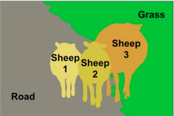
ROAD, SHEEP, SHEEP, SHEEP, GRASS

(Differentiate instances)

In the example above Instance Segmentation distinguishes between the three sheep instances.

The output is like in semantic segmentation where we have this pixel wise accuracy but here for each of these objects we also want to say which pixels belong to that object.

Method

The idea is to get region and classification predictions (for each object) and then apply semantic segmentation onto each of these regions.

Mask R-CNN

Kaiming He, Georgia Gkioxari, Piotr Dollar, Ross Girshick: Mask R-CNN (2018)

And this ends up looking a lot like Faster R-CNN.

So it has this multi-stage processing approach where we take our whole input image, that whole input image goes into some convolutional network and some learned region proposal network that's exactly the same as Faster R-CNN and now once we have our learned region proposals (input image goes through CNN - RPN) then we project those proposals onto our convolutional feature map just like we did in Fast and Faster R-CNN.

But now rather than just making a classification and a bounding box for regression decision

for each of those boxes we in addition want to predict a segmentation mask for each of those region proposals. So now it kind of looks like a semantic segmentation problem inside each of the region proposals that we're getting from our region proposal network.

Mask R-CNN Architecture
Kaiming He Georgia Gkioxari Piotr Dollar Ross Girshick: Mask R-CNN

After we do this RoI aligning to warp our features corresponding to the region of proposal

into the right shape, then we have two different branches.

First branch at the top looks just like Faster R-CNN and it will predict classification scores telling us what is the category corresponding to that region  proposal or alternatively whether or not it's background. And we'll also predict some bounding box coordinates that regressed off the region proposal coordinates.

Mask R-CNN Architecture in detail

Image source: Stanford University School of Engineering - Convolutional Neural Networks for Visual Recognition - Lecture 11 | Detection and Segmentation

And now in addition we'll have this branch at the bottom which looks basically like a semantic segmentation mini network which will classify for each pixel in that input region proposal whether or not it's an object. This Mask R-CNN architecture just kind of unifies Faster R-CNN and Semantic Segmentation models into one nice jointly end-to-end trainable model.

It works really well, just look at the examples in the paper. They look kind of indistinguishable from ground truth.

Pose Estimation

Mask R-CNN also does pose estimation. You can do pose estimation by predicting these joint coordinates for each of the joints of the person.

Mask R-CNN can do joint object detection, pose estimation, and instance segmentation.

And the only addition we need to make is that for each of these region proposals we add an additional little branch that predicts these coordinates of the joints for the instance of the current region proposal.

Addition for pose estimation

Image source: Stanford University School of Engineering - Convolutional Neural Networks for Visual Recognition - Lecture 11 | Detection and Segmentation

As another layer has been added (another head coming out of the network) we need to add another loss to our multi-task loss.

Because it's built on the Faster R-CNN framework it runs relatively close to real time so this is running something like 5fps on a GPU because this is all sort of done in the single forward pass of the network.

Training

How much training data do you need?

All of these instant segmentation results were trained on the Microsoft Coco data set. Microsoft Coco is roughly 200,000 training images. It has 80 categories that it cares about so in each of those 200,000 training images it has all the instances of those 80 categories labeled. So there's something like 200,000 images for training and there's something like I think an average of five or six instances per image. So it actually is quite a lot of data. And for Microsoft Coco for all the people in Microsoft Coco they also have all the joints annotated as well so this actually does have quite a lot of supervision at training time. It is trained with quite a lot of data.

Training: Future improvements

One really interesting topic to study moving forward is that we kind of know that if you have a lot of data to solve some problem, at this point we're relatively confident that you can stitch up some convolutional network that can probably do a reasonable job at that problem but figuring out ways to get performance like this with less training data is a super interesting and active area of research.
That's something people will be spending a lot of their efforts working on in the next few years.

Reference:

Stanford University School of Engineering - Convolutional Neural Networks for Visual Recognition - Lecture 11 | Detection and Segmentation - YouTube

Kaiming He Georgia Gkioxari Piotr Dollar Ross Girshick: Mask R-CNN (2018)

Semantic Segmentation

Input

• image (pixels)
• list of categories

Goal

Each pixel in the image to be classified (to be assigned a category label).

Don't differentiate instances (objects), only care about pixels.

Output

• Every input pixel is assigned a category
• Pixels of each category are painted with the same color e.g. grass, cat, tree, sky
• If two instances of the same object are next to each other, entire area will have the same label and will be painted with same color

Method

Approach #1: Sliding Window 

Approach #1 is to use sliding window where we are moving a small window across the image and apply DNN classification to determine the class of the crop which is then assigned to the central pixel of the crop.

This would be very computationally expensive as we'd need to classify (push crop through CNN) separate crop for each pixel in the image.

This would also be very inefficient for not reusing shared features between overlapping patches. If two patches overlap then the convolutional features of these patches will end up going through the same convolutional layers and we can actually share a lot of computation when applying this to separate passes or applying this type of approach to separate patches of the image. 

Approach #2: CNN, layers keep spatial size

Using fully convolutional network where whole network is a giant stack of convolutional layers with no fully connected layers where each convolutional layer preserves the spatial size of the input:

input image --> [conv] --> output image

• input 3 x H x W
• convolutions D x H x W: conv --> conv --> conv --> conv--> 
• scores: C x H x W (C is the number of categories/labels)
• argmax ==> Predictions H x W

Final convolutional layer outputs tensor C x H x W.

The size of the output image has to be the same as the input image as we want to have classification for each pixel, output image has to be pixel-perfect, with sharp and clear borders between segments.

All computations are done in one pass. 

Using convolutional layers which are keeping the same spatial size as the input image is super expensive and would take lots of memory for the huge number of parameters required (high resolution input image, input in each layer has multiple channels...).

Approach #3: CNN, downsampling + upsampling

Design network as a bunch of convolutional layers, with downlsampling and upsampling of the feature map inside the network:

input image --> [conv --> downsampling] --> [conv --> upsampling] --> output image

Downsampling: 

• spatial information gets lost
• e.g. max pooling, strided convolution

Upsampling: max unpooling or strided transpose convolution.

Training

Put classification loss at every pixel at the output, take an average through space and train it through normal back propagation.

Data

Creating training set is expensive and long manual process. Each pixel has to be labelled. There are some tools for drawing contours and filling in the regions.

Loss Function

Loss function: cross-entropy loss is computed for each pixel in the output and ground truth pixels; then sum or average is taken over space or mini-batch.

Problem

Individual instances of the same category are not differentiated. This is improved with Instance Segmentation.

References:

Stanford University School of Engineering - Convolutional Neural Networks for Visual Recognition - Lecture 11 | Detection and Segmentation - YouTube

Object Detection with SSD

SSD (Single Shot Multibox Detector) is a method for object detection (object localization and classification) which uses a single Deep Neural Network (DNN). Single Shot means that object detection is performed in a single forward pass of the DNN.

This method was proposed by Wei Liu et al. in December 2015 and revised last time in December 2016: SSD: Single Shot MultiBox Detector.

Objective

Fast Object Detection.

Method

The SSD network, built on the VGG-16 network, performs the task of object detection and localization in a single forward pass of the network. This approach discretizes the output space of bounding boxes into a set of default boxes over different aspect ratios and scales per feature map location. At prediction time, the network generates scores for the presence of each object category in each default box and produces adjustments to the box to better match the object shape. Additionally, the network combines predictions from multiple features with different resolutions to naturally handle objects of various sizes. [source]

Here are some key points from the paper's abstraction:

• SSD uses single deep neural network
• SSD discretizes the output space of bounding boxes into a set of default boxes over different aspect ratios and scales per feature map location

BK: note here that different aspect ratios and scales are not applied to anchor boxes in the image but feature map

• At prediction time, the network generates scores for the presence of each object category in each default box and produces adjustments to the box to better match the object shape. Additionally, the network combines predictions from multiple feature maps with different resolutions to naturally handle objects of various sizes. 
• Our SSD model is simple relative to methods that require object proposals because it completely eliminates proposal generation and subsequent pixel or feature resampling stage and encapsulates all computation in a single network. This makes SSD easy to train and straightforward to integrate into systems that require a detection component. 
• Experimental results on the PASCAL VOC, MS COCO, and ILSVRC datasets confirm that SSD has comparable accuracy to methods that utilize an additional object proposal step and is much faster, while providing a unified framework for both training and inference. Compared to other single stage methods, SSD has much better accuracy, even with a smaller input image size. For 300×300 input, SSD achieves 72.1% mAP on VOC2007 test at 58 FPS on a Nvidia Titan X and for 500×500 input, SSD achieves 75.1% mAP, outperforming a comparable state of the art Faster R-CNN model. 

SSD Framework

Image source: Wei Liu, Dragomir Anguelov, Dumitru Erhan, Christian Szegedy, Scott Reed, Cheng-Yang Fu, Alexander C. Berg: SSD: Single Shot MultiBox Detector

We know that deeper Conv layers in CNNs extract/learn more complex features.
Feature maps preserve spatial structure of the input image but at lower resolution.

Lecture 11: Detection and Localization


If we take some CNN (like ResNet) pretrained for image recognition (image classification) and remove its last FC layers we'll get as its output a feature map as described above.

Now we can do something which YOLO does on the image - divide feature map into a grid cells and apply equidistant detector which predicts anchor boxes.



--------------
Given our input image (3 * H * W) you imagine dividing that input image into some coarse S * S grid, and now within each of those grid cells you imagine some set of B base bounding boxes (e.g. B = 3 base bounding boxes like a tall one, a wide one, and a square one but in practice you would use more than three). These bounding boxes are centered at each grid cell.

Now for each of these grid cells (S x S) network has to predict two things:

• for each of these base bounding boxes (B): an offset off the base bounding box to predict what is the true location of the object off this base bounding box. 
• This prediction has two components:
• bounding box coordinates: dx, dy, dh , dw
• confidence
• So the final output has B * 5 values
• classification scores for each of C classes (including background as a class)

At the end we end up predicting from our input image this giant tensor:

S * S * (B * 5 + C)

So that's just where we have B base bounding boxes, we have five numbers for each giving our offset and our confidence for that base bounding box and C classification scores for our C categories.

So then we kind of see object detection as this input of an image, output of this three dimensional tensor and you can imagine just training this whole thing with a giant convolutional network.

And that's kind of what these single shot methods do where they just, and again matching the ground truth objects into these potential base boxes becomes a little bit hairy but that's what these methods do.
--------------

Architecture

SSD has two components:

• base (backbone) model
• SSD head

Backbone model:

• usually a pre-trained image classification network as a feature extractor from which the final fully connected classification layer has been removed; such NN is able to extract semantic meaning from the input image while preserving the spatial structure of the image albeit at a lower resolution
• VGG-16 or ResNet trained on ImageNet 

SSD head:

• one or more convolutional layers added to the backbone
• outputs are interpreted as the bounding boxes and classes of objects in the spatial location of the final layers activations

SSD vs YOLO Network Architecture
Image source: Wei Liu et al.: "SSD: Single Shot MultiBox Detector"

Examples

Tensorflow Object Detection API comes with pretrained models where ssd_inception_v2_coco_2017_11_17 is one of them.

TensorRT/samples/opensource/sampleUffSSD at master · NVIDIA/TensorRT · GitHub

TensorFlow implementation of SSD, which actually differs from the original paper, in that it has an inception_v2 backbone. For more information about the actual model, download ssd_inception_v2_coco. The TensorFlow SSD network was trained on the InceptionV2 architecture using the MSCOCO dataset which has 91 classes (including the background class). The config details of the network can be found here.

Logo detection in Images using SSD - Towards Data Science
TensorFlow Object Detection API with Single Shot MultiBox Detector (SSD) - YouTube


ssd_mobilenet_v1_coco_2017_11_17

References:

Wei Liu, Dragomir Anguelov, Dumitru Erhan, Christian Szegedy, Scott Reed, Cheng-Yang Fu, 

Alexander C. Berg: SSD: Single Shot MultiBox Detector

TensorRT UFF SSD

RattyDAVE/pi-object-detection: Raspberry Pi Object detection.

https://github.com/weiliu89/caffe/tree/ssd

https://machinethink.net/blog/object-detection/

SSD : Single Shot Detector for object detection using MultiBox

13.7. Single Shot Multibox Detection (SSD) — Dive into Deep Learning 0.7.1 documentation

Understanding SSD MultiBox — Real-Time Object Detection In Deep Learning

How single-shot detector (SSD) works? | ArcGIS for Developers

(20) Is SSD really better than YOLO? - Quora

Review: SSD — Single Shot Detector (Object Detection)

SSD object detection: Single Shot MultiBox Detector for real-time processing

What do we learn from single shot object detectors (SSD, YOLOv3), FPN & Focal loss (RetinaNet)?

References

Sunday, 14 March 2021
Sunday, 19 January 2020