Unsupervised Machine Learning

Monday 27 December 2021

Unsupervised Machine Learning

Data is, by default, unlabeled. Labeling data is manual (or somewhat automated) process, thus timely and expensive. Unsupervised machine learning uses unlabeled data (raw, cheap, widely available) for model training. Nevertheless, this comes with the cost of unsupervised learning requiring higher volumes of data for the training if comparing to supervised learning.

Typical use cases for unsupervised ML:

Clustering
Anomaly Detection
Dimensionality Reduction

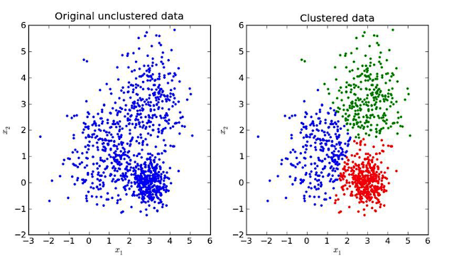
Clustering

Unsupervised learning algorithms extract features and patterns from unlabeled data which can then be used to label and group together data points that share same or similar features. This is known as clustering and is one of typical problems solved by unsupervised learning.

image source: KDNuggets

Clustering algorithms:

k-means clustering
neural networks

hypothesis function is a mapping from input space back into this input space
the goal of an unsupervised learning loss function is to measure the difference between the hypothesis function and the input itself

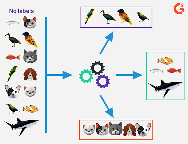
Example: Image set clustering

Each cluster contains images which have the same object in them. Model does not know the name of that object, that it is e.g. bird. It only knows (learns) that objects in each cluster share the same/similar features. We might only need to set in advance the number of clusters we want to get.

In supervised learning, if we have a labeled dataset which contains images of birds, fish and mammals, our model will learn to identify if the image contains a bird, a fish or a mammal. In unsupervised learning, model will learn to distinguish and separate images that share same/similar features and it would group them in three clusters but it would not know that in one cluster are birds and in another fish for example, it would just know that there are three (or maybe even more) types of objects.

image credits: Devin Pickell, g2.com

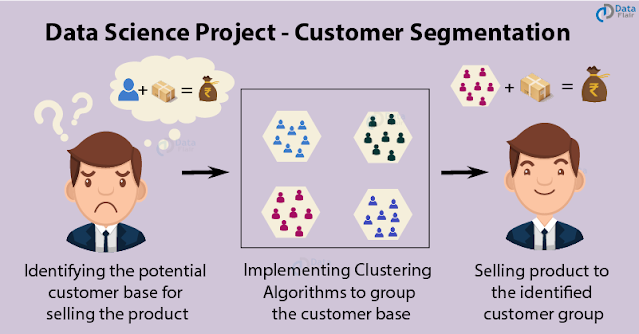
Example: Customer segmentation

Each cluster contains customers of some differentiable profile. This helps in e.g. targeted marketing.

image source: data-flair.training

Example: Spam detection

Unsupervised learning algorithm can analyze huge volumes of emails and uncover the features and patterns that indicate spam (and keep getting better at flagging spam over time).

Anomaly Detection

Another type of problems solved by unsupervised learning is anomaly detection. The goal here is to find abnormal data points. Model is trained to detect if data point has some unusual features.

Example: Fraud detection (Anomaly Detection)

Fraudulent transactions tend to involve larger sums of money. Fraud only occurs with transfers and cash-out transactions.


image credit: Shirin Elsinghorst, codecentric.de

Class 0 is normal transaction. Class 1 is fraudulent transaction.

Dimensionality Reduction

Data dimensionality refers to feature space. Each data point can be defined as a vector in N-dimensional space where N is number of features. Some features are more and some less important, in a way how much do they contribute in differentiating data points. The more features, the more complex model is, the more time and storage is required for its training and inference. The idea here is to reduce number of features without losing the semantic meaning of the data. E.g. bird can still be distinguished from other animals by recognising that it has features like beak, wings and a tail but eye color or feather color pattern is not important.

Some dimensionality reduction techniques:

Independent Components Analysis (ICA)
Principal Components Analysis (PCA)

Sometimes, before applying k-means clustering, a dimensionality reduction is applied on data.

Principal Component Analysis (PCA)

Transforms data from d-dimensional to p-dimensional feature space where p < d. It first finds the dimension of the highest variance (e.g. direction where the data is most spread out) - principal component. Data points are then projected onto this dimension. Small amount of information gets lost but overall data integrity is not changed.

PCA is based on reducing correlation (linear dependence) between features. If two features are linearly dependent, we can derive value of one feature if value of the another one is known. PCA removes this redundancy by projecting a set of linearly dependent features into a smaller set of new, uncorrelated features.

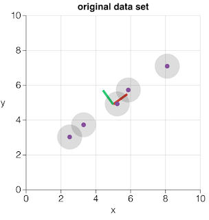Original data points are in 2-dimensional feature space. Features are denoted as x and y.

PCA finds the direction along which values have the highest variance. It is a red diagonal in our case.

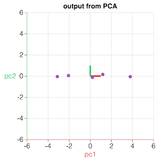Data points are projected onto component which carries the highest variance. That principal component becomes a newly derived feature. The next principal component (pc2) which carries the most variance is the one defined by the line perpendicular to the direction of pc1.

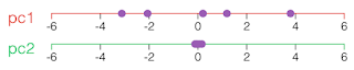As pc2 exhibits low variance, this component does not carry much information (that helps differentiating data points). It can be ignored (small amount of information is lost) thus reducing the feature space to a single dimension.

image credits: V. Powell, setosa.io

Example: Solution to “Cocktail Party” problem

Dimension Reduction via Independent Components Analysis (ICA) is used to extract independent sources of audio signal from a recording which contains mixed signals.